Deriving Muon

Boston, 7 Mar 2025

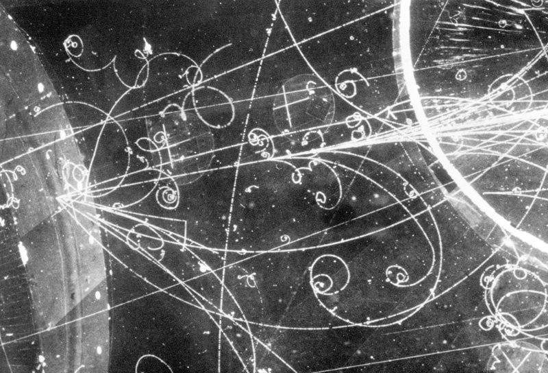
Particle tracks in a bubble chamber. Fermilab.

We recently proposed Muon: a new neural net optimizer. Muon has garnered attention for its excellent practical performance: it was used to set NanoGPT speed records leading to interest from the big labs.

What makes Muon particularly special to me is that we derived the core numerical methods from an exact theoretical principle. This is in contrast to popular optimizers like Adam, which have more heuristic origins and often converge slower than Muon. In this post, I will walk through a derivation of Muon. I hope this will provide context that may help researchers extend the methods to new layer types and beyond.

While this post focuses on the theory behind Muon, I recommend checking out Keller’s post to learn more about the algorithm—including the substantial ingenuity that went into making the implementation run fast.

What is Muon?

Muon is an optimizer specifically designed for \(\mathsf{Linear}\) neural network layers. By \(\mathsf{Linear}\), I mean layers that take an input vector \(x\) and multiply by a weight matrix \(W\) to return an output vector \(y = W x\). There is also an expectation that the vectors \(x\) and \(y\) are “dense” activation vectors, meaning the entries are close to unit size. This latter requirement separates the \(\mathsf{Linear}\) layer from, say, an \(\mathsf{Embedding}\) layer that takes one-hot inputs.

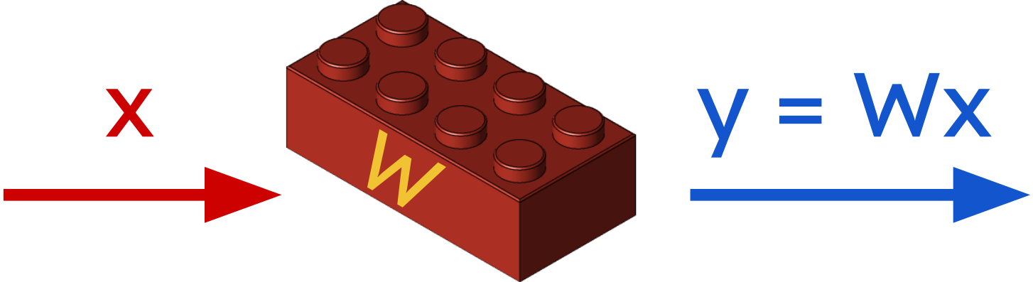
The Linear layer is an important building block in neural networks.

While it may seem suprising—and it is certainly non-standard—to use different optimizers for different layer types, this is part of our broader mission to “modularize” the theory of deep learning. The idea is to break up the architecture into building blocks, derive theory and algorithms for each separate piece, then work out how to glue the pieces together at the end.

The Lego Transformer. Thanks to Idan Shenfeld for letting me play with this.

To handle individual layers, our idea is to normalize the weight updates in a clever way so that, given the structure of the inputs, the weight updates automatically induce a desirable effect on the outputs. As a community, we have invested so much effort into thinking about how to normalize the activations: think batch norm, layer norm, RMS norm, etc. Why not also consider how the weights and weight updates influence the activations?

Muon in four steps

Okay, time to focus! Back to Muon! In this post, we are going to derive the following version of the Muon update rule:

To unpack this expression:

• the scalar parameter \(\eta\) sets the step size;
• \(\texttt{fan-out}\) and \(\texttt{fan-in}\) are the dimensions of the weight matrix \(W\);
• \(\nabla_W \mathcal{L}\) is the gradient of the loss \(\mathcal{L}\) with respect to the weights \(W\);
• \(\mathrm{NewtonSchulz}\) is an orthogonalization routine—I’ll explain later!

In practice, Muon uses a slightly different dimensional pre-factor, but I’d actually expect the one here to scale better. The other difference is that in the Python implementation we apply Newton-Schulz to the momentum (essentially a running average of gradients) instead of to the gradient itself.

Step 1: Metrizing the linear layer

First, we will metrize the linear layer: that is, we will equip the inputs, weights and outputs with relevant measures of size. This will help us control the sizes of these quantities and also their updates through training.

In a neural network, a linear layer is intended to map from “dense” input vectors to “dense” output vectors. By “dense”, we mean that the average size of the entries is around one. We can quantify the average size of the entries using the root-mean-square (RMS) norm:

where \(d\) is the dimension of the vector \(v\). The second equality states that the RMS norm is a normalized version of the Euclidean norm. If all the entries of a vector are \(\pm 1\), then the RMS norm of the vector is one.

Now, we ask the question: how can a weight matrix affect the RMS norm of its outputs, given that we know the RMS norm of its inputs? To answer this question, we need a tool known as the operator norm of a matrix.

The operator norm tells us how much a matrix can stretch an input vector.

The RMS-to-RMS operator norm is defined as the maximum amount by which a matrix can increase the average entry-size of its inputs:

The second equality says that the RMS-to-RMS operator norm is equivalent to a normalized version of the spectral norm \(\|\cdot\|_*\) of the matrix. The spectral norm is the largest singular value of the matrix.

Step 2: Perturbing the linear layer

We train a neural network by updating the weight matrices. These weight updates lead to changes in the layer outputs. In this step of the derivation, we will show that the operator norm of the weight update allows us to bound how much the outputs can change in response.

Consider applying an update \(\Delta W\) to the weights of a linear layer. The resulting change in output \(\Delta y\) is given by:

We can bound the size of the output perturbation \(\|\Delta y\|_{\text{RMS}}\) in terms of the size of the weight perturbation \(\|\Delta W\|_{\text{RMS} \to \text{RMS}}\) just by applying the definition of the RMS-to-RMS operator norm:

A good way to think about this inequality is as the very simplest example of a more general idea: connecting the size of the weight update to the amount of change induced in the resulting function.

Step 3: Dualizing the gradient

For the third step in the derivation, we consider choosing a weight update to maximize the linear improvement in loss \(\mathcal{L}\) while maintaining a bound on the amount that the outputs can change in response. The rationale is that if the weight update makes the layer outputs change too much, this could de-stabilize the overall network. In symbols, we would like to solve:

To construct a proxy for solving this problem, we can apply inequality \((\star)\) from the previous section to switch from controlling the size of the output change to directly controlling the size of the weight update itself. If the input has size \(\|x\|_{\text{RMS}} \leq 1\), we obtain the following problem as a proxy:

In words: let’s minimize the linearized loss while controlling the size of the weight update. Seems reasonable! We refer to solving \((\dagger)\) as “dualizing the gradient” under the RMS-to-RMS operator norm. If the gradient has singular value decomposition (SVD) given by \(\nabla_W \mathcal{L} = U \Sigma V^\top\), then \((\dagger)\) is solved by:

In words: we keep the singular vectors of the gradient but throw away the magnitudes of the singular values. This corresponds to “orthogonalizing” the gradient. A sanity check that this is a sensible operation is to see that the update \((\S)\) encourages inequality \((\star)\) to hold tightly, meaning that the update tries to saturate the bound on the change in output. Later on, we will see that this property leads to learning rate transfer across width.

One challenge remains before we can turn the update rule \((\S)\) into a workable algorithm. Orthogonalizing the gradient would naïvely require computing the SVD of the gradient, which seems too expensive to be practical at large-scale. But fear not, we shall develop a workaround!

Step 4: Dualizing fast via Newton-Schulz

The final step in the derivation is to work out a fast means of performing the gradient orthogonalization step:

We proposed performing this step via a so-called “Newton-Schulz” iteration. The main idea underlying the technique is that odd matrix polynomials \(p(X)\) “commute” with the SVD. In other words, for an odd polynomial

applying \(p\) to the matrix \(X\) is equivalent to applying \(p\) directly to the singular values of \(X\) and then putting the singular vectors back together:

To orthogonalize a matrix, we would like to set all the singular values to one. Since all the singular values are positive, we can think of this as applying the sign function to the singular values. While the sign function is an odd function, it is unfortunately not a polynomial. However, we can produce low-order odd polynomials that converge to the sign function when iterated. A simple example (Kovarik, 1970) is the cubic polynomial:

To visualize this cubic, we plot the scalar function \(y = p_3(x)\) on the left. And on the right, we plot the cubic composed with itself 5 times to obtain \(y = p_3\circ p_3 \circ p_3 \circ p_3 \circ p_3(x)\). Notice that the iterated cubic starts to resemble the sign function in the neighbourhood of the origin:

In fact, \(p_3 \circ p_3 \circ p_3 \circ \cdots \circ p_3 (\Sigma)\) will converge to \(\mathrm{sign}(\Sigma)\) so long as the initial singular values are normalized to be less than \(\sqrt{3}\). We call this a “Newton-Schulz iteration” following the terminology of Nick Higham.

All that remains is to combine update rule \((\S)\) with a Newton-Schulz iteration, et voilà—we have derived our version of Muon!

Payoff #1: Fast training with automatic learning rate transfer

Phew, that was a lot of work! But we are finally ready to see the payoff. The first payoff is that dualizing the gradient under the RMS-to-RMS operator norm leads to both fast and scalable training. The following plot shows that dualizing the gradient under the RMS-to-RMS norm leads to learning rate transfer across width and a much better final loss than training with Adam.

Training MLPs on CIFAR. Dualized training is both faster than conventional training and leads to automatic learning rate transfer across width. SP stands for standard parameterization and μP stands for maximal update parameterization. Thanks to Laker Newhouse for running this experiment.

The reason that dualizing the gradient in the RMS-to-RMS operator norm leads to learning rate transfer across width is that the dualized updates encourage inequality \((\star)\) to hold tightly, meaning that the updates try to induce a controlled amount of RMS output change independent of width.

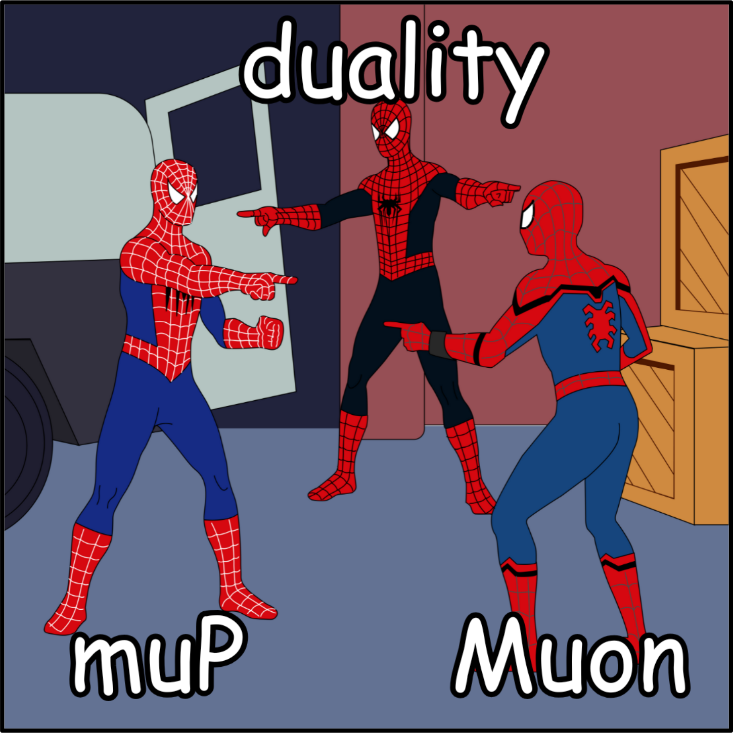
There was already a well-known technique for achieving learning rate transfer across width: the so-called maximal update parameterization, or μP for short. We have shown that the μP learning rate scaling is obtained automatically by dualizing the gradient in the “correct” norm. As such, I believe that μP and Muon are really two sides of the same coin.

Payoff #2: Simpler numerical properties

A more subtle payoff is that Muon has somewhat simpler numerical properties than other optimizers. To visualize this, I ran an experiment inspired by Jesus et al. (2020) where we watermark an initial weight matrix with the letter “a” and then track the erasure of the watermark as we train. This allows us to visually tell how much the weights move through training.

In the following plot, we show the final visibility of the watermark after training with both dualized and non-dualized updates over a range of different learning rates. As can be seen, not only does dualized training converge faster, but it also leads to faster erasure of the watermark.

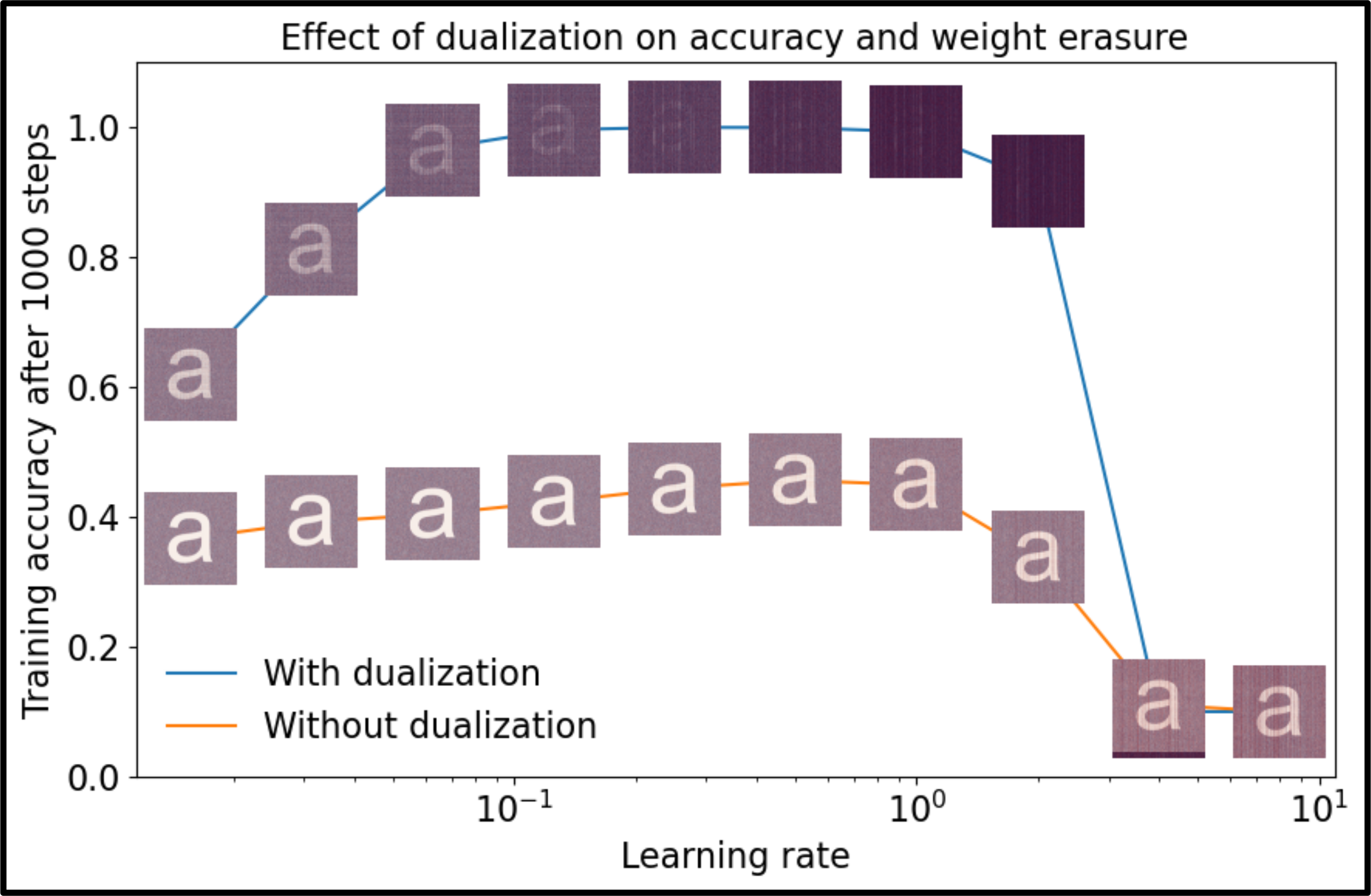
Dualized training converges faster and erases the watermark faster. I wrote up a thorough explanation for this effect in the Modula docs.

I believe this experiment underscores how properly metrized and dualized deep learning can have an impact on the kinds of number systems and precision levels we use to represent and train neural networks.

This effect also has theoretical implications. Many researchers took the observation that the weight entries seem to hardly move in standard training as evidence that it was safe to study deep learning in a linearized regime around the initialization. This is the so-called neural tangent kernel (NTK) regime. But the weight erasure experiment shows that in dualized training the weights can move substantially from their initial values.

Related work

There have been a couple of papers from the past decade that also had the idea of orthogonalizing and dualizing the gradients in deep learning optimization. I highly recommend checking out the following two papers:

• Stochastic spectral descent (2015) by David Carlson, Edo Collins, Ya-Ping Hsieh, Lawrence Carin & Volkan Cevher.
• Duality structure gradient descent (2017) by Thomas Flynn.

We had the idea for spectral norm dualization independently of these papers. That said, our main theoretical novelties in hindsight are to propose using the Newton-Schulz iteration to enable very fast orthogonalization on GPUs, and to propose using the RMS-to-RMS operator norm instead of the spectral norm, leading to learning rate transfer across width.

It is also important to credit the proponents and developers of the Shampoo optimizer. The kinds of numerical routines used inside Shampoo are what made me realize back in August 2024 that orthogonalization could be feasible on GPUs at scale. Check out the following papers:

• Scalable Second Order Optimization for Deep Learning (2020) by Rohan Anil, Vineet Gupta, Tomer Koren, Kevin Regan & Yoram Singer.
• A Distributed Data-Parallel PyTorch Implementation of the Distributed Shampoo Optimizer for Training Neural Networks At-Scale (2023) by Hao-Jun Michael Shi et al.

Finally, I must mention the AlgoPerf competition. It feels like it breathed fresh life into the field of deep learning optimization, and spurred me to take a closer look at Shampoo. Check out the two write-ups from the team:

• Benchmarking Neural Network Training Algorithms (2023) by George Dahl et al.
• Accelerating neural network training: An analysis of the AlgoPerf competition (2025) by Priya Kasimbeg et al.

If you are interested to find more papers on this topic, I am collating a reading list on the Modula docs. Let me know if I should add anything!

Conclusion: The geometry of neural networks

To summarize, in this post:

• we derived a version of Muon in four steps;
• we showed the resulting method leads to scalable and fast training;
• we showed the resulting method has novel numerical properties.

I want to finish the post by discussing what I see as the bigger picture here.

For a long time, neural networks felt to me like inscrutable beasts. A tangled web of complicated interacting effects: high-dimensional spaces, tensors, compositionality, stochasticity… You name it! The analytical tools we had at our disposal felt inadequate in the face of this complexity.

I am now feeling more optimistic that we can in fact disentangle this complicated web and formalize a neural network as a set of precise mathematical concepts with understood interactions. I see this as the long-term goal of the Modula project. I have been lucky to work with some of the best scientists and mathematicians in the world to get to this point.

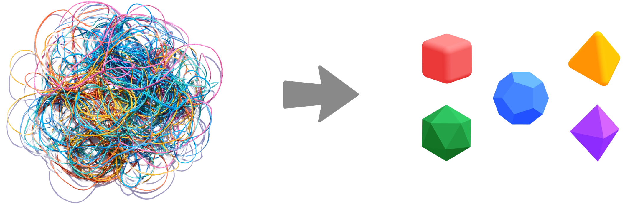
Can we distentangle neural networks into precise mathematical concepts?

One of these important mathematical concepts is the idea of geometry. There is an old and deep connection between optimization and geometry, with different notions of distance leading to different optimization theories:

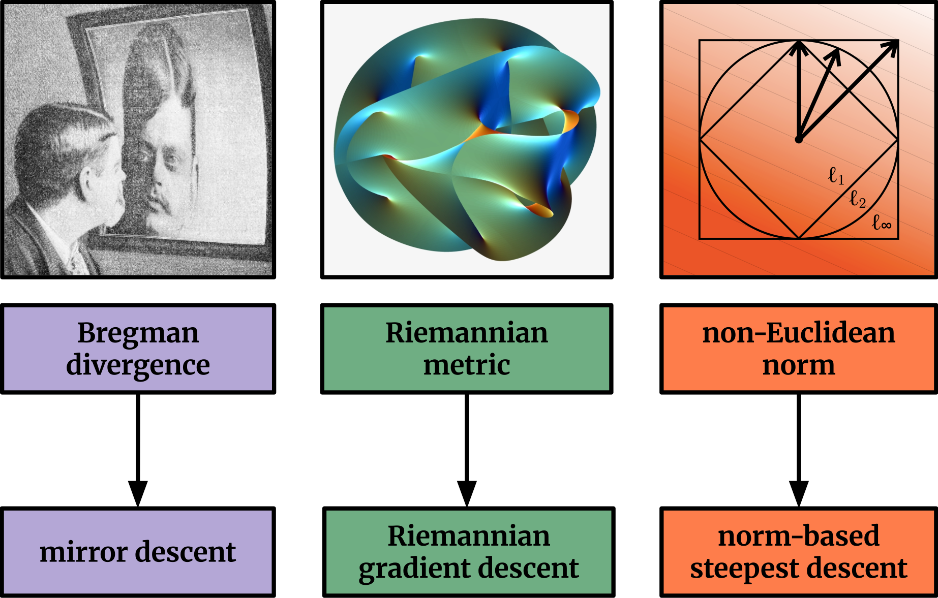
Different notions of distance lead to different optimization theories.

In Muon, we are exploiting the geometry of a matrix that acts as a linear operator between RMS-normed vector spaces. In particular, we build on a geometric connection between distance in weight space and distance in function space. We have already put significant work into extending this idea to general network architectures: starting with my work on deep relative trust and leading up to our most recent work on the modular norm and modular duality. I am excited to see where this work goes from here!

Citing this blog post

To cite this blog post, you can use the following BibTeX entry:

@misc{bernstein2025deriving,
  author = {Jeremy Bernstein},
  title = {Deriving Muon},
  url = {https://jeremybernste.in/writing/deriving-muon},
  year = {2025}
}

The official citation for the Muon optimizer is:

@misc{jordan2024muon,
  author = {Keller Jordan and Yuchen Jin and Vlado Boza and Jiacheng You and Franz Cesista and Laker Newhouse and Jeremy Bernstein},
  title = {Muon: An optimizer for hidden layers in neural networks},
  url = {https://kellerjordan.github.io/posts/muon/},
  year = {2024}
}

Python code for Muon is available here.

Acknowledgements

I am grateful to Phillip Isola, Laker Newhouse, Isha Puri and Akarsh Kumar for helpful discussions and feedback on this blog post. I am extremely grateful to Phillip Isola for granting me the freedom to pursue this research. Thanks to Jyo Pari for doing the lego transformer photo shoot with me.