Getting to the bottom

Los Angeles, 6 Apr 2020

Despite the tremendous progress made in deep learning research over the last decade, we are still working out the mathematical principles underlying precisely how neural nets learn. Given their relationship to the brain—and their burgeoning presence in modern technology—it is an exciting time to work on the foundational properties of neural networks.

In a recent paper written by myself, Arash Vahdat, Yisong Yue and Ming-Yu Liu, we propose a mathematical formula that measures the distance between two neural networks. In particular, we focus on two deep networks with the same architecture but different synaptic weights. Whilst this concept might seem esoteric, here are a few concrete reasons you might care about it:

• you want to know “how far” you can perturb the synapses of a network before destroying its properties. Knowing this is important for both stable learning and network compression.
• you want to make sure that the network does not “move too far” in response to any one training example. Knowing this is important for the generalisation theory of Bousquet and Elisseeff, as well as for techniques in differential privacy.
• you want to measure the “width” of the minimum that learning settles into. Some machine learning researchers believe this concept is important for understanding generalisation.

In our paper, we focused on the implications of our distance for stable learning, and that is what we shall cover in this post. We leave the other implications as interesting avenues for further research.

Before we get down to the mathematical nitty-gritty, we shall first provide a hands-on demonstration of our main idea.

Hands-on deep learning

For the purposes of this demonstration, we have restricted to networks with two inputs and one output. This lets us visualise the response of any neuron as a 2-dimensional heatmap, where the \((x,y)\) coordinates correspond to the network input, and the color corresponds to that neuron’s response. Now, please build your network!

We want to train your network to classify a dataset of inputs as orange or blue. The batch size controls how many training examples we will show to your network each training step. Please choose your dataset and batch size!

The time has come for your network to learn something. Choose your learning algorithm and step size, then hit play!

Hopefully your network found a good decision boundary. The spiral dataset is a little tricky, so you may need to adjust the learning settings or network architecture a couple of times.

Now that we’ve trained your network, it’s natural to ask: how stable is it? One way we can assess this is by seeing how much noise we can we add to the network weights before the decision boundary breaks down. For each layer, we shall scale the noise so that its norm is a percentage of the norm of the weights for that layer. Hit the red button to try it out!

In our experiments, we found that small relative perturbations to each layer have little effect, whereas large relative perturbations distort the decision boundary a lot. What did you find?

At this point, take a bit of time to play and explore the neural network’s properties. One idea to get started: try training a depth 1 and depth 20 network on the checkerboard dataset. Perturb the weights with 20% noise. Which function is more stable?

Formalising the idea

At the end of the previous section, we introduced the idea that the strength of a perturbation to a neural network’s weights is governed by its layerwise relative size. To get a sense of the generality of this idea, try bursting this bubble by adding layerwise relative noise to the GAN that generated it:

Whilst the idea was explored in this 2017 paper by Yang You, Igor Gitman and Boris Ginsburg, it was largely missed by the rest of the research community (including us!)—possibly because the idea was not formalised.

To formalise the idea, let’s pick a mathematical notation. We shall pass an input \(x\) through the \(L\) layers of the neural network. We use \(\phi\) to denote the network’s nonlinearity, and \(W\) the weights. \(W\) is really a tuple over the \(L\) layers: \(W=(W_1,W_2,...,W_L)\). Then we can denote the output of the network as:

\[f(W;x):= \phi \circ W_L \,\circ \,... \circ \,\phi \circ W_1 (x).\]

Before we head to our final destination, let’s take our notation for a spin. A well known mathematical object in deep learning theory is the “input-output sensitivity” of the network. This asks, how stable is the network output \(f(W;x)\) to perturbations \(\Delta x\) to the input \(x\)? The standard result is that:

\[\frac{\|f(W;x+\Delta x)-f(W;x)\|}{\|\Delta x\|} \leq \prod_{l=1}^L \|W_l\|_{*}.\]

If you haven’t seen the spectral norm \(\|\cdot\|_*\) before, don’t worry—it’s just a way of measuring the size of a matrix. In words, the result says: the sensitivity of the network output to its input (lefthand side) is bounded by the product of the size of each layer’s weights (righthand side). This explains why it’s a good idea to regularise the size of the weight matrices during training—it smoothens out the network function by making it less sensitive to input variations.

Given that input-output sensitivity asks how sensitive \(f(W;x)\) is to variations in its argument \(x\), it becomes natural to ask the same question for variations in its other argument \(W\). Let’s perturb the weights by a tuple \(\Delta W = (\Delta W_1,...,\Delta W_L)\). After a slightly tricky calculation in our paper, we found that the “weight-output sensitivty” is given by:

\[\frac{\|f(W+\Delta W;x)-f(W;x)\|}{\|f(W;x)\|} \lessapprox \prod_{l=1}^L \left[1 + \frac{\|\Delta W_l\|_F}{\|W_l\|_F}\right] -1.\]

Notice the similarity between this inequality and the input-output sensitivity: both depend on a product over the network layers, reflecting the product structure of the original network. A key difference is that this result depends on the relative size of the perturbation to each layer. We call it the distance between two neural networks.

Stable learning

Since training a neural network involves perturbing the weights to adjust the output, it is fairly intuitive that the “weight-output sensitivity” that we derived should play its part. But to see exactly how, we need to find the right way to conceptualise first order optimisation. In particular, we shall propose a view that is—to our knowledge, and despite its simplicity—novel.

First order optimisation involves minimising a cost function \(\mathcal{L}(W)\) by pushing the network parameters “downhill” along the negative gradient direction. But the gradient \(g(W) := \nabla_W \mathcal{L}(W)\) is only a local description of the function, and it will break down if we move too far. Another way to see this is via the first order Taylor expansion:

\[\mathcal{L}(W+\Delta W) \approx \mathcal{L}(W)+g(W)^T\Delta W.\]

This is a local approximation, meaning that if the perturbation \(\Delta W\) grows too large, then the gradient changes and the approximation breaks down. The idea of gradient descent is to descend the first order Taylor expansion with a small enough step size that the approximation remains good. We may express this principle formally as:

\[\displaylines{\min_{\Delta W} \left[\mathcal{L}(W)+g(W)^T\Delta W \right]\qquad\qquad\qquad\qquad\qquad\\ \qquad\qquad \text{such that}\,\frac{\|g(W+\Delta W) - g(W)\|}{\|g(W)\|}< 1.}\]

Whilst we present this principle as a maxim, it may be obtained more rigourously from the fundamental theorem of calculus. We omit the details so as not to obfuscate the core idea.

At this point, the missing ingredient is an efficient way to estimate the relative breakdown in gradient for neural networks. Here’s a picture to give you an idea of a couple different ways the gradient might break down:

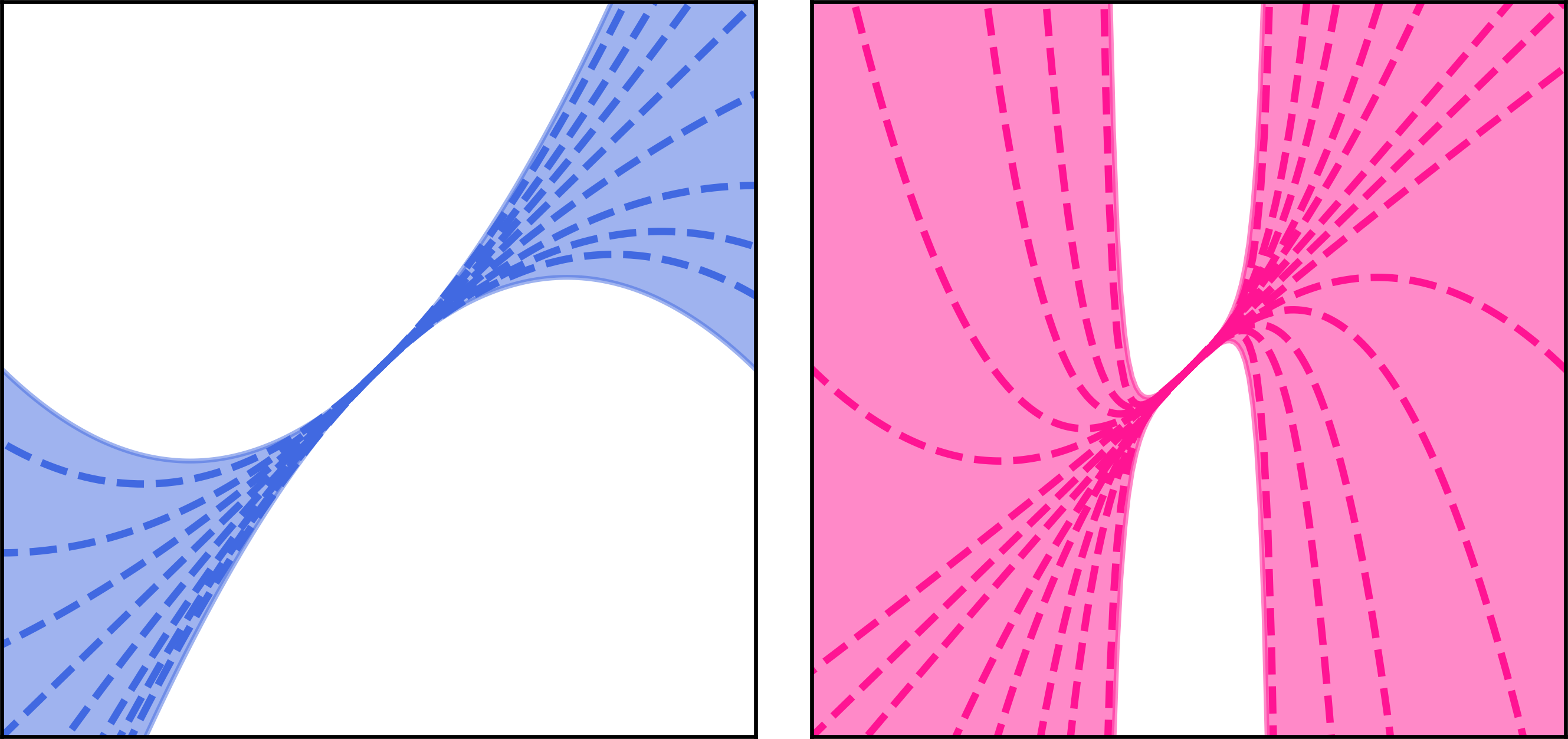
It might break down very smoothly, like the functions on the left. Or suddenly, like the functions on the right. In our paper, we provide theoretical and empirical evidence that for a multilayer perceptron the gradient breakdown is governed by the weight-output sensitivity, as follows:

\[\frac{\|g(W+\Delta W) - g(W)\|}{\|g(W)\|} \lessapprox \prod_{l=1}^L \left[1 + \frac{\|\Delta W_l\|_F}{\|W_l\|_F}\right] -1.\]

So we have our gradient reliability estimate, and we are ready to design an optimiser!

Fromage 🧀

Assembling the pieces, we arrive at the following training procedure for neural networks—written out in a layerwise form:

\[\displaylines{\min_{\Delta W} \left[\mathcal{L}(W)+\sum_{l=1}^L g_l^T\Delta W_l \right]\qquad\qquad\qquad\qquad\qquad\\ \qquad\qquad \text{such that}\prod_{l=1}^L \left[1 + \frac{\|\Delta W_l\|_F}{\|W_l\|_F}\right] -1 < 1.}\]

The minimand ensures we move downhill, and the constraint prevents us moving too far. We would really like a closed form algorithm rather than this constrained optimisation procedure. By inspection, a good candidate is:

\[\Delta W_l = - \eta \cdot g_l\cdot \frac{\|W_l\|}{\|g_l\|},\]

where \(\eta\) is a small positive number. This update is good because it clearly points in the right direction, and the gradient reliability estimate reduces to \((1+\eta)^L - 1\) which is indeed smaller than one for small enough \(\eta\).

When combined with a second order stability correction that we explain in the paper, we call this algorithm “Fromage”, short for Frobenius matched gradient descent. In our experiments, the algorithm held certain practical advantages:

• it worked well across a range of problems, from GAN training to image classification to NLP. These are domains where deep learning practitioners typically employ a host of different algorithms;
• it greatly eased the choice of an appropriate learning rate. For Fromage the learning rate is meaningful—it is the layerwise relative perturbation strength. A value of 0.01 worked out of the box for most problems.

Quite late in our research we realised that the Fromage algorithm is quite similar to the LARS algorithm and its followup LAMB. Whilst there are differences, such as our second order stability correction, we prefer to think that we are laying out the theoretical foundation for LARS and LAMB.

Horizons

I believe that the key contribution of this work is the conceptual shift that it makes. We trade talking about phenomenological terms like “vanishing and exploding gradients”—a deep learning favourite—for more mathematically conventional objects like “weight-output sensitivity”.

As mentioned in the introduction, this shift could be useful for building a better understanding of generalisation in deep neural networks. It could also have a practical impact on private learning, where the goal is to prevent the network from learning too much from any single training example.

Early in my PhD I came to believe that the challenge of theoretical deep learning research is not to prove advanced theorems but rather to work out the right set of modelling assumptions for neural networks. In a mathematical sense, we are still finding the right axioms—theorems can come later! I hope that this work is a step in that direction.

Acknowledgements

The neural net visualisations in this post were built using Tensorflow Playground by Daniel Smilkov and Shan Carter. The bursting bubble was generated by BigGAN.